Creating a Surface Area Calculator in Google Sheets
In my post about the benefits and the possibilities of using spreadsheets in middle school math classes, here are the instructions that I used to get my students started on spreadsheets. If you want it to download the PDF then click this link HERE!
You can find it electronically by following this link: https://pcauley.clarify-it.com/d/kvdxee
Creating a Surface Area Calculator in Google Sheets
This quick guide will show you how to program your very own surface area calculator in Google Sheets (or any spreadsheet program).

Step 1 – Create a new Google Sheet
Head over to drive.google.com and log in (if you’re note already).
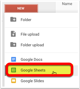
Then click on New and a drop down menu will appear.
Now click on Google Sheets.
Step 2 – Set up your spreadsheet
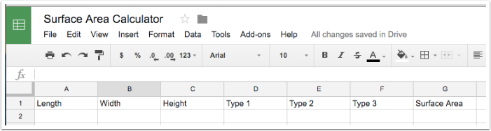
Now it is time to set up your spreadsheet.
Notice that each cell has a coordinate or cell reference. The columns are labeled by letters and the rows are numbered.
In these cells put this information:
- A1 = Length
- B1 = Width
- C1 = Height
- D1 = Type 1
- E1 = Type 2
- F1 = Type 3
- G1 = Surface Area
Step 3 – Input your dimensions
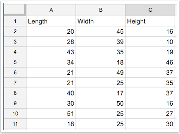
Now that we have the spreadsheet set up it is time to start entering in your data.
Put in the length, width and height for each 3-D object.
You can find the dimensions we used by clicking this link HERE!
Step 4 – Calculate the different types
We know there are three types of sides in a rectangular prism, so we need to find those types. However, if you just type the equation into a cell, it will not work. You have to enter it a special way in order for it to work. Check out the special characters below.
- You must start each equation with an equal sign =
- Addition uses the plus sign +
- Multiplication uses an asterisk
*
We can add numbers directly into the cell, but we can also tell the spreadsheet to add cells which will make it much faster for us.
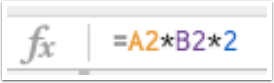
So our first equation in cell D1 we will multiply the information in A2 to the information in B2 and then multiply it by two. The equation will look like the image below.
Now make your own equations for Type 2 and Type 3.
*REMINDER – ALWAYS USE AN EQUAL SIGN FIRST BEFORE TYPING IN THE EQUATION*
Step 5 – Replicate the equation
You do not have to type in the equation over and over again. There is a way that you can replicate the equation over and over by just clicking and dragging.
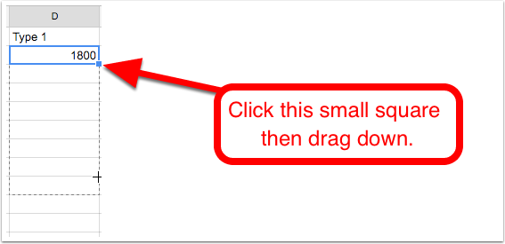
- Now select the cell with the equation in it.
- You will notice a small square in the bottom right hand corner of the cell
- Click and drag that little square down.
Now do this for the Type 2 and Type 3 columns.
Step 6 – Calculating Surface Area
Now that we have calculated the different types, it is time to calculate the surface area.
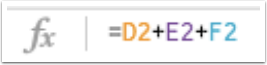
Make sure you are in cell G2.
Now we need to add the data in cells D2, E2 and F2.
Your equation should look like the image below.
Step 7 – Replicate the Surface Area formula
Now replicate that equation like you did for Type 1, Type 2 and Type 3.
Congratulations!
You should have a working spreadsheet that will automatically calculate the surface area for you correctly everytime.
Remember you can do this with any spreadsheet program like Excel, LibreOffice or Numbers (for Mac).
![]()
Source: IT Babble Blog and Podcast