Making a GCF and LCM calculator in Google Sheets
Howdy everyone! It’s been a looooong time but I’m back and ready to post more frequently (at least I hope)
Today is a little tutorial for just about any middle school (probably a fifth grade too) math class. It shows you how to create a “calculator” in Google Sheets (or any spreadsheet program – looking at you Excel) of how to automatically calculate greatest common factor (GCF) and least common multiple (LCM).
It’s pretty straight forward so enjoy!
If you want a PDF of the instructions click HERE!
If you want a clean e-version click HERE!
Finding the greatest common factor and the least common multiple is not particularly hard but it is a necessary skill in math. When dealing with smaller numbers, it can be very easy and even done mentally. However, when dealing with larger numbers it can pose a real problem.
This guide will show you how to make that in Google Sheets. This guide can also be applied to Microsoft Excel, Libre Office Calc and any other decent spreadsheet program.
Step 1 – Create a new spreadsheet
In order to do this, we need to create a new spreadsheet.
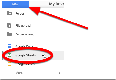
Go to drive.google.com and click on the New button.
Then select Google Sheets.
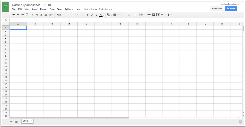
This will create a new spreadsheet which looks like this.
Name your Google Sheet
It is always a good idea to name your files, so you can easily find it again.
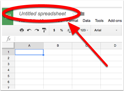
To do this, click where it says Untitled spreadsheet.
Then type in an appropriate name. I am calling mine GCF – LCM Calculator
Step 2 – Set up your spreadsheet
Now that the spreadsheet has been created and named, it is time to set it up.
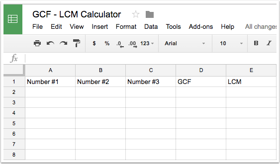
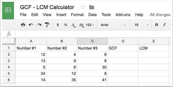
Make your spreadsheet look like mine:
- Cell A1 = Number #1
- Call B1 = Number #2
- Cell C1 = Number #3
- Cell D1 = GCF
- Cell E1 = LCM
*NOTE: THOSE RECTANGLES THAT MAKE UP THE SPREADSHEET ARE CALLED CELLS*
Step 3 – Add some numbers
In this part I just added some numbers.
Use the same numbers I have so you can compare your final results with mine.
To enter the numbers, just click on the cell and type them in.
Step 4 – Calculating the GCF
We are now going to enter a formula to have the spreadsheet automatically calculate the greatest common factor for us.
Anytime we enter an equation we MUST start with an equal sign =
We will type this formula is cell D2:
=gcd(A2,B2,C2)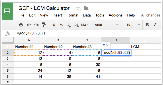
Here is what is happening.
We are telling the spreadsheet to find the GCF that is what this part of the formula does.
=gcdThe GCD means greatest common divisor which works for us. We need the parenthesis to help the spreadsheet what to look for and the letters and numbers refer to the cells.
=gcd(A1,B1,C1)So it is looking for the GCD (or GCF) for the numbers in cells A1, B1 and C1.
Our first result should be a 2.
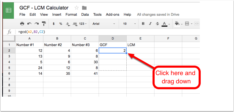
Step 5 – Replicate the formula
All spreadsheets have a nifty trick where you can replicate the formula so you don’t have to type it in again.
Click cell D2 and you should see a little blue box (the one my arrow points to).
Click and drag that down to cell D6.
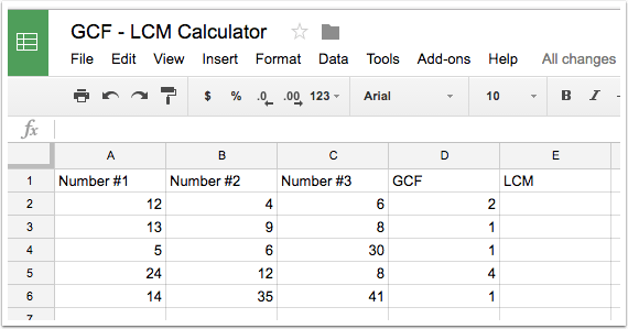
Here is what your spreadsheet should look like now.
Step 6 – Calculate the LCM
Now that we’ve done the GCF, it is time to write the formula in for the LCM.
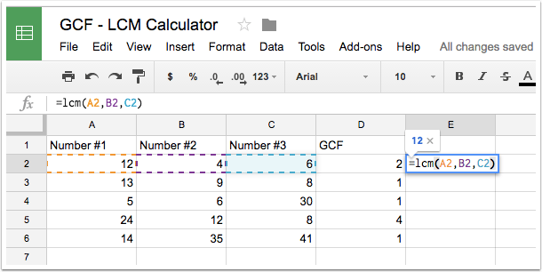
In cell E2 we will type in the following formula.
=lcm(A2,B2,C2)Then hit enter.
Replicate the formula
Now go ahead and replicate the formula as we did before.
Check out the GIF below.
Congratulations
Now you can change all the numbers and it should calculate the GCF and the LCM instantly for you.
Enjoy 
![]()
Source: IT Babble Blog and Podcast