Students making their own gradebook in Google Sheets
In my last post I talked about the importance of grades being transparent for all stake holders involved. One idea I recommend is having students build their own gradebook in Google Sheets (or any spreadsheet program). This gives them significantly more insight in how grades actually work, behave and gives the student more ownership with their own grades.
However, not all teachers may have the experience or knowledge on how to lead their students to do this – in fact doing it step by step with a class is tough, so I went ahead and made a quick guide.
Note this guide does not cover weighted grades.
To download a PDF of this guide click HERE!
On find it online HERE!
Otherwise here it is in all its glory.
Google Sheets – Making your own gradebook
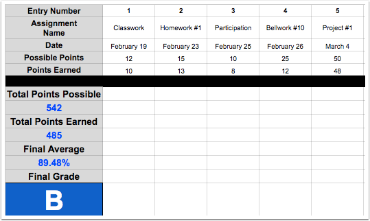
This guide will help you create your very own functional gradebook so you can keep track of your own grades and have a better understanding of how grades are calculated, figured and how impactful each grade truly is.
We will be entering in 20 separate assignments, projects and tests into this sample gradebook. Feel free to add more or less as you see fit.
Let’s begin.
Step 1 – Open up a blank Google Sheet
Go to drive.google.com and sign in.
Then click the New button (on the left hand side).
A drop down menu should appear and from there select Google Sheets.

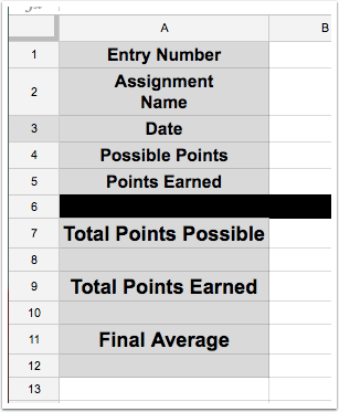
Step 2 – Set up the first half of your gradebook.
You want your gradebook to have two halves. The top half will have all the individual assignments. The second half will be the final calculations and final percentage (or grade if you are courageous enough).
Write this information in each corresponding cell.
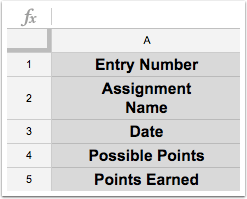
- A1 = Entry Number
- A2 = Assignment Name – (see if you can figure out how I wrote the word Name below the word Assignment)
- A3 = Date
- A4 = Possible Points
- A5 = Points Earned
Step 3 – Add the dividing line
To better separate the top half from the bottom half we will add a black dividing line.
This is very easy to do.
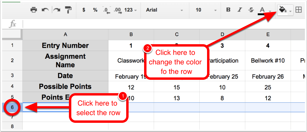
Click the Row Number 6 – this will highlight the whole row.
Then click the paint bucket button in the toolbar and select the color black. This will make a black line separating the two sections.
Step 4 – Create the Totals section
This section will tell us how many total points there are and what our final average is.
This section is very easy to set up.
Add this information in each corresponding cell.
- A7 = Total Points Possible
- A9 = Total Points Earned
- A11 = Final Average
We will add equations to A8, A10 and A12 later, so leave them blank for now.
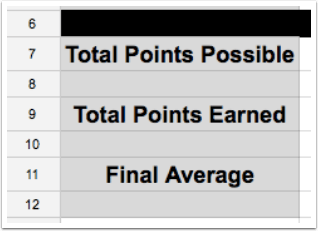
This is what your spreadsheet should look like now.
I have some done some formatting like centering text, adding a grey background to the cell, increasing the size of the font. Format your gradebook however you like.
Step 5 – Adding Entry Numbers
This is a simple step. We want to add entry numbers. To do this start typing in 1, 2, 3, 4 . . . 20
Again, I centered them and made them bold but you can format as you like.

Step 6 – Adding Assignment Names, Date, Possible Points and Points Earned
Now we can start adding in assignments.
Make up the assignment name, date, possible points and points earned for your 20 assignments.
*Helpful Tip: You can automatically format the date by selecting the dates and then clicking on Format —> Numer —> More Formats —> More date and time formats*

Step 7 – Total points
Now that we have a bunch of data in the top half, we can start to work on some calculations on the bottom half.
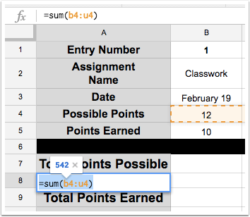
In cell A8 we need to calculate the Total Points. Here we will need to add all the cells in Row 4 – the Possible Points row
In cell A8 we will type this equation: =sum(b4:u4)
Step 8 – Total points earned
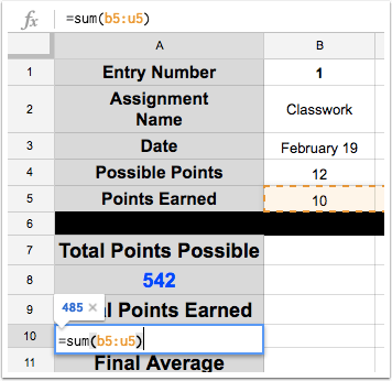
Now we will add up all of our total points earned.
In cell A10 type this equation: =sum(b5:u5)
Step 9 – Final average
Now that we have our total points and our total points earned – we can calculate our final average.
To find our final percentage we need to divide the total points earned into the total points possible.
In cell A10 write this equation: =A10/A8
You should see a decimal. That’s OK – we will fix that next.
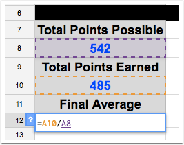
Now I see a decimal but changing it into a percentage is very easy.
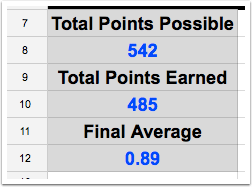
Highlight the cell with the decimal in it.
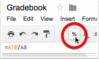
On the toolbar there is a percentage button (%). Click that
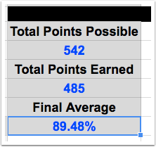
Now you have a final percentage!
Optional steps
If these 9 steps were easy – test yourself by adding this functionality to your gradebook.
- You can use conditional formatting to highlight assignments that are 0’s
- Create a final grade that changes based on the final average (this is completely new)
- Create a row to show averages for each assignment
- Create conditional formatting for each assignment to highlight low grades
- Create a way to lookup assignments to get all their information quickly (challenging)
Good luck!