Google Forms & Sheets – Olympic Scoring – Part 3
The journey continues and this marks the hump point of this series. Just a quick recap. In Part 1 I wrote about how I was using Google Forms and Sheets to create an auto calculating scorebook and the services and skills I used. In Part 2 I talked about how I created the Google Form and got it to do what I needed it to do. We also had Google set up a spreadsheet with our data from the form as well.
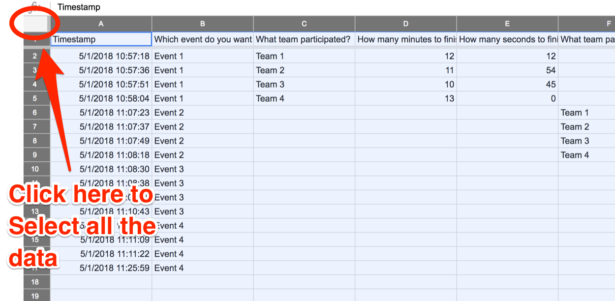
Here we are in Part 3. Here we are going to set up specific worksheets for each event. Before we start adding functions to a worksheet let’s take a look at the data we have. I went ahead and filled out the form. I have 4 teams and 4 events.
That may be a little small so click this link to get a view only peak at the data. Again, this was all organized by Google automatically. The data is nice, it is organized and it makes perfect sense. What we are going to do now is create additional worksheets in this file to help us filter the data and allow us to organize it for each specific event.
Just a note. If you get stuck and frustrated don’t worry – especially if you have never done any work in a spreadsheet. Stick with it, be patient with yourself and reach out if you need any assistance. Learning something new isn’t always easy.
OK, now we’re ready.
Naming that data
From the Form Responses 1 worksheet we are going to name all this data. This makes it easier to reference it back when using functions in other worksheets. To do this click the empty box below the fx symbol near the top left hand side of the screen. This will select all the data.
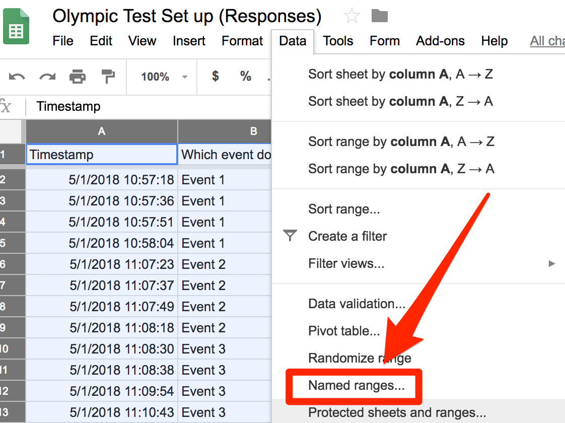
Now we need to name it. To do this select Data from the top most menu bar. Then select Named ranges…
Now give it a very simple name with no spaces. Spaces apparently will break it. I also like to keep it lower case. I don’t know why, maybe it is just me but I always make my named ranges lower case.
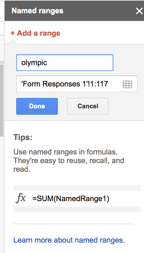
I called this data olympic. It is simple, easy to remember and hard to misspell.
Create a new worksheet
This might sound like we are going to create a whole new file but no. Spreadsheets have the ability to add different worksheets. Not being a spreadsheet master I feel this is a way to reference other data from other worksheets while at the same time filtering or showing specific data in a particular context.
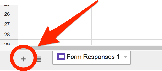
Doing this is super easy. Open up your spreadsheet. You can get to it through the Google Form Responses page by clicking on the Google Sheets icon (see Part 2 of this series for a screenshot). Then click on the plus button down in the bottom left hand corner of your screen.
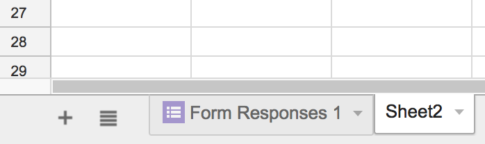
If all goes well you should see this! You can rename any sheet by double clicking on its name in the tab. I am calling mine Event 1.
Now to go to that sheet (if it didn’t do it automatically) by clicking on the tab, like a browser tab. You will see a blank worksheet but that will change shortly. You will notice that the columns are labeled as letters and the rows are all labeled as numbers. This is used so we can reference specific cells known as cell reference.
We will start our journey in cell B1. Here we will add a Query function.
Query
The Query function will allow you to pull specific data from the From Responses 1 worksheet. There is a reason we are putting it in cell B1 and not A1 but that will become clear later on. So we only want the Event 1 data in this worksheet.
Here is what you will need to type in cell B1:
=query(olympic,"SELECT B,C,D,E WHERE B='Event 1'",0)
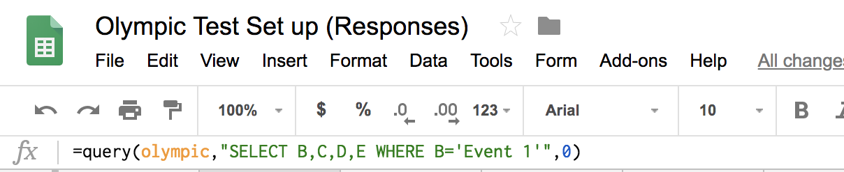
Let’s break down this formula so you can understand what is happening.
- The = sign is what is needed to start all functions. This lets the spreadsheet know that it is performing an action and not just holding data.
- The word olympic refers back to all the data on the Form Responses 1 sheet.
- The comma breaks the function into a different part.
- Select B,C,D,E tells us that we are only going to display the data in these columns.
- WHERE B=’Event 1 tells us that column B must have those exact words and based on that will show the information in those rows corresponding to columns B,C,D,E
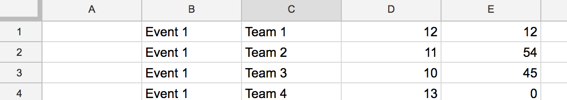
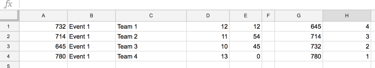
When all is done here are the results!
Total seconds
I am sure there is a function that will sort based on two columns but I do not know it. However, I do know how to sort values in one column. So what we are going to do is convert the minutes and seconds to seconds in Column A.
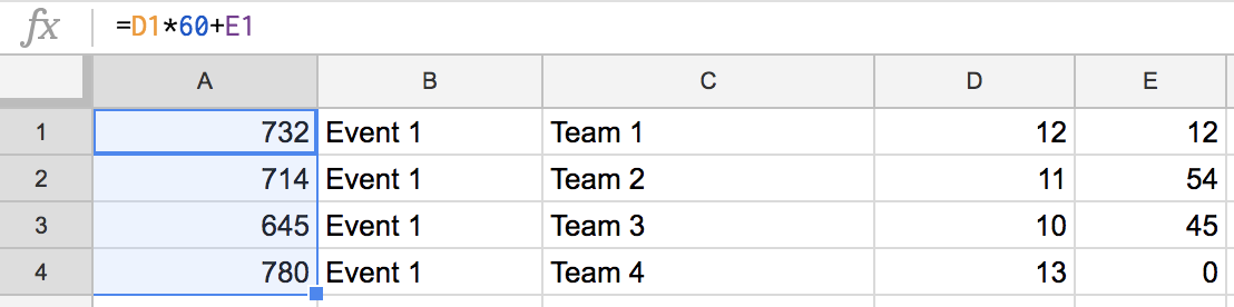
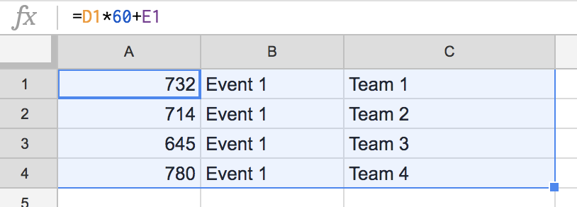
To do this I typed in this function in A1:
=D6*60+E6
What this does it take the value in cell D6 (the number of minutes) and multiplies it to 60 (converting minutes to seconds) and then adds the value in E6 (the number of seconds) to that total.
Now copy that formula for the other teams. Be sure to change D6 and E6 to D7 and E7 and so on and so on.
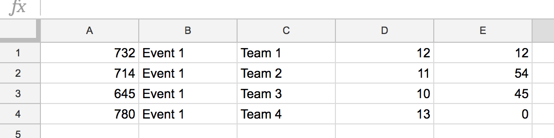
Here is what you should have now.
Ranking with the small function
Now we need to rank them or put them in order from fastest to slowest. I am sure there is a way to do this more efficiently but as I have mentioned earlier, I just don’t know how and so I am working with what I know and what I can do.
First I want to highlight the total seconds column and name that range, I don’t want all the data in this worksheet just the total seconds in Column A so that is all I highlight. I called this data event1sec.
Then in Column G (I want to leave column F alone just for aesthetics) I will type this formula:
=small(event1sec,1)
- The small function returns the smallest value in a set of data.
- event1sec is the data it is looking a.
- 1 this means I want the smallest set of data
So for the next row down here is what you would type:=small(event1sec,2)
The 2 means it wants the second smallest number in that data set.
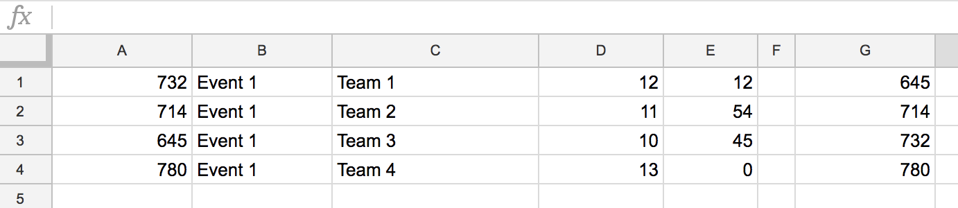
So this is what your spreadsheet should look like now.
vlookup
We are nearly done!
In column H, I will simply add the scores. I just type in the numbers into the cell manually. There is a way to write an if statement to get this automatically but this seems a little simpler for me.
H1 = 4
H2 = 3
H3 = 2
H4 = 1
Now that we have the numbers ranked you could look back and match up the numbers mentally but it would be best if the country is next to its score. We will be using the vlookup function here and we will be putting that function in cell I1 (that is “i” like Iceland).
Before we add the vlookup we need to name another range. Here I will be highlighting A1 to C4.
I will name this range event1pts. The process is the same as before.
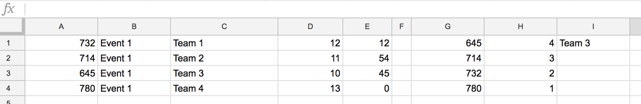
Now let’s add the vlookup function in cell I1 (as I mentioned before).
=vlookup(G1,event1pts,3,0)
Now here is what is happening with this formula.
- G1 is the number it is looking up.
- event1pts is the data that vlookup is looking at.
- 3 is looking at the third column (so in this case column C of that data set) and that is what is will be shown depending on the value in G1
- 0 means that it wants an exact match
Here is what that should look like.
Now for the next row (I2) you will want to type this function:
=vlookup(G2,event1pts,3,0)
Then use G3 and finally G4.
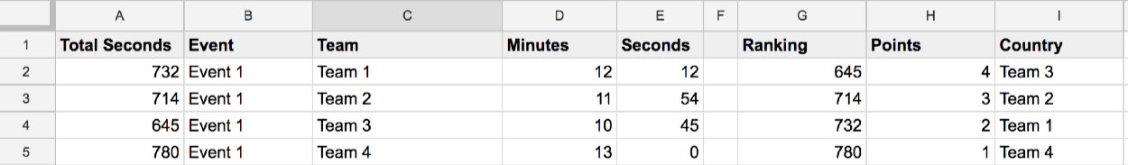
Now I went ahead and inserted a row at the top and here is the final worksheet.
Duplicate and update
This is the last step and it is pretty easy. We can duplicate this worksheet and only change one function to make it all work for the different events!
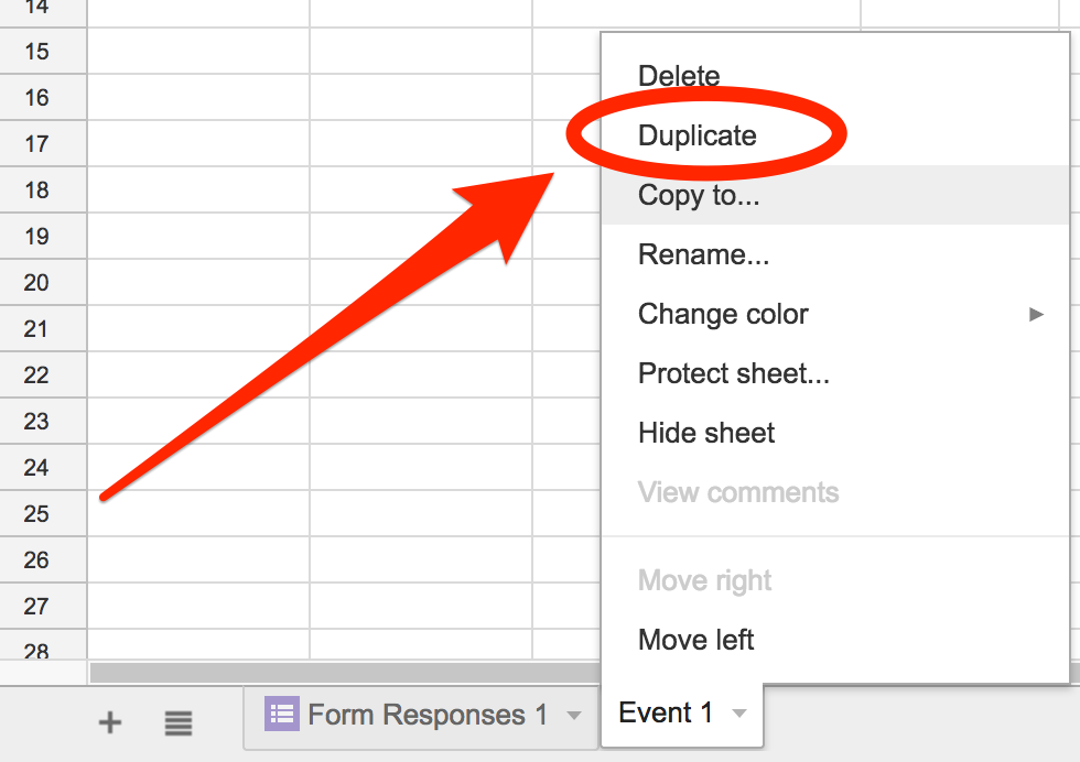
Here we go, in the worksheet tab at the very bottom left hand corner of your screen right click the tab for Event 1.
You should see a menu appear. From here select Duplicate.
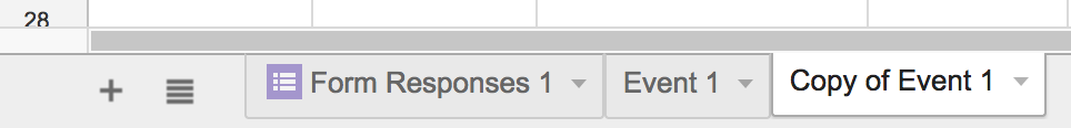
A new tab will appear and it will contain exactly the same data as the Event 1 worksheet.
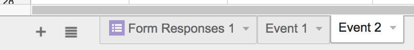
From here I will rename the Copy of Event 1 tab to Event 2.
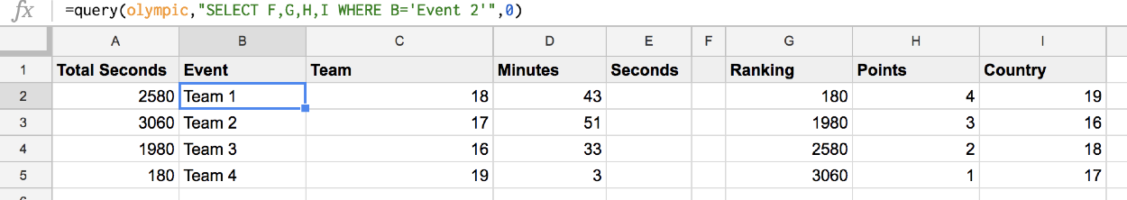
Now I will go to the Event 2 worksheet and find my Query function. It should be in cell B2.
In this function I will change B,C,D,E to B,G,H,I. B stays the same because that column holds the which event it is in the Form Responses 1 worksheet.
Then I will change WHERE B=’Event 1’ to WHERE B=’Event 2’.
Here is an image of the new formula.

=query(olympics,"SELECT B,F,G,H WHERE B='Event 2'",0)
And magically the data should update! Awesome.
Now let’s do it for Event 3 and 4.
Duplicate Event 2
Rename it to Event 3
Change the query function to this:=query(olympics,"SELECT B,I,J,K WHERE B='Event 3'",0)
Duplicate Event 3
Rename it to Event 4
Change the query function to this:=query(olympics,"SELECT B,L,M,N WHERE B='Event 4'",0)
Parting notes
If you’ve been able to follow along and all of your sheets look great well done. If not keep at it. This is a lot to take in and again, if you’ve never dabbled into spreadsheets this could take a while to wrap your head around. I’ve tried to write this post in a way that I feel most people can follow but again, it is almost 2000 words and there are a lot of steps. If there is something you don’t quite get please email me at: patrickcauley@gmail.com and I’ll do my best to help.
Part 4 – Setting up the team worksheets coming soon!
Source: IT Babble Blog and Podcast