Google Forms & Sheets – Olympic Scoring – Part 5

It has been a long road and we are finally at the finish line. This post will talk about how to total everything so you can see who wins without calculating anything! We will also talk about limitations to this form and how it is not perfect. If you are new to this series please check the first 4 parts.
- Part 1 – The overview
- Part 2 – Setting up the Google Form
- Part 3 – Setting up the event worksheets
- Part 4 – Setting up setting up the countries
Now open up your worksheet and let’s get into the fun!
Make a new worksheet
We are going to make a new worksheet. To do this click the )+ button in the bottom left hand corner of your Google Sheet.
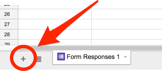
It will make a new tab and a blank worksheet. If the tab is not where you would like it to be simply click and drag it to the desired location. I am naming this worksheet totals
The first thing I will do is set up the worksheet. So there will be no functions (yet) just typing some text into some cells.
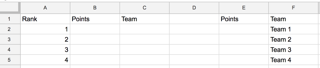
Now I left Column D empty for aesthetic reasons – no other reasons. The other columns are set up for a specific reasons which we will soon see.
Referencing the points
In column E we will be referencing the total points. You could just type them in, but I like referencing them back to their original cell. Here is how we do that.
- Type in the = sign
- Click to the Team 1 worksheet
- Click on the link with their total points
- Then hit the Enter key
Check out the video below.
Named range
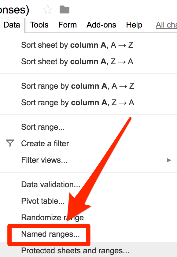
Now that we have all the teams and their total points we need to name a range. I will highlight from E2 to F5. Then I will select Data from the menu bar and click on Named ranges…
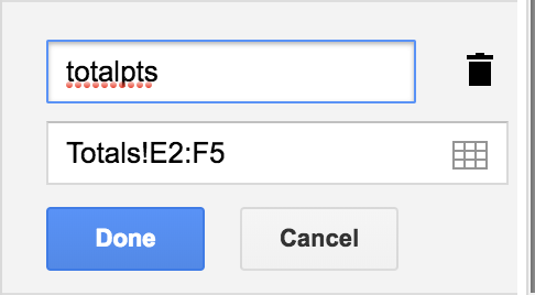
I will call this data totalpts. Remember when naming data you cannot use spaces.
Large function
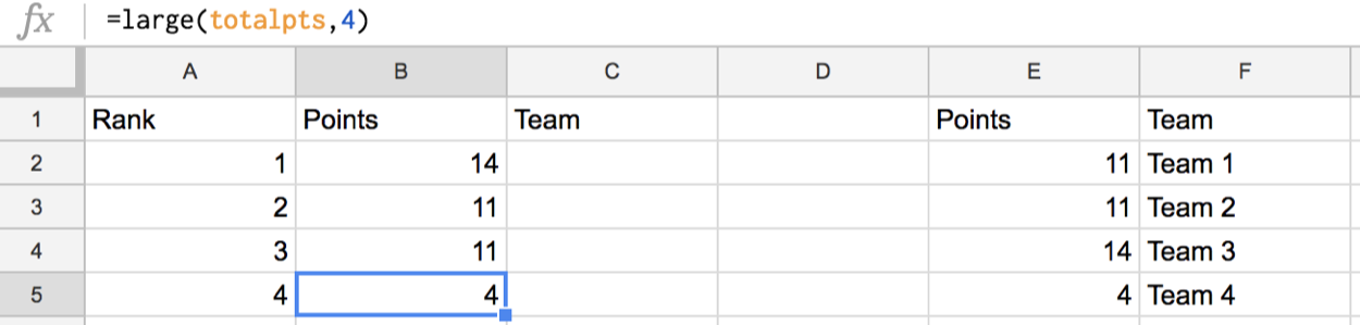
Now that we have that done it is time to start using some functions to rank the teams. In cell B2 we will be using the large function. This does the opposite of the small function we used in Part 2. So basically this will show us the largest value in a set of data. Here is what we type in cell B2:
=large(totalpts,1)
- The totalpts is the set of data we just named
- The 1 means to show the largest of the set of data
Now we will repeat this function for cell B3 and type this:
=large(totalpts,2)
And so on all the way dow to cell B5. When you’re done here is what you should have.
vlookup
We are nearly done. Now we will utilize the vlookup function again and we will be using this in column C. What this will do is to look at the number in column B and then match that number up with the team name.
In cell C2 here is what we will type:=vlookup(B2,totalpts,2,0)
- B2 is the value vlookup is looking for
- totalpts is the set of data where vlookup is looking
- 2 refers to the second column of the data, in this case column F
- 0 Means we want an exact match.
In cell C3 here is what I need to type:
=vlookup(B3,totalpts,2,0)
Here is what mine looks like.
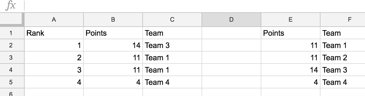
Uh? Patrick? What happened to second and third place?
OK, here is the time we will talk about imperfections. Obviously ties are not handled very well with the vlookup function. I have no idea how to solve this simply (or even complexly). If you are well versed with spreadsheets please leave solutions below! 
Ties are a problem with this set up that is obvious.
Another issue here is testing the form. You could build this entire spreadsheet, all the worksheets without any data. It is possible, but I prefer to add a bunch of bogus data, build the form so I can see that it is all working properly and then wipe the data out. Not ideal but you want to make sure your hardwork has been done correctly and that once real data gets in there you know it will be handled properly.
Well that is the scoreboard in all its glory. If you have ideas on where it can be improved or what can be added let me know by adding in the comments below!
Source: IT Babble Blog and Podcast