Google Forms & Sheets – Olympic Scoring – Part 4

Please check out Part 1, Part 2 and Part 3 to get caught up. If you are just jumping in now and have little spreadsheet experience you may feel a little lost.

Last post we made all the worksheets for all the eventa. In this post we are going to make worksheets for each country or team. Lucky for us, there is a lot less “moving parts” here. These sheets will simply compile all the results for all the events for each team and then total those points up.

Named Ranges

Before we start making worksheets for each team or country we need to name some ranges and we will do that back in the event worksheets. So I will open up my spreadsheet and go to the Event 1 worksheet.

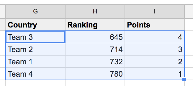
I am not going to add or change anything. I am simply going to highlight some data and then give it a name. So on the Event 1 worksheet I will highlight G2 to I5.

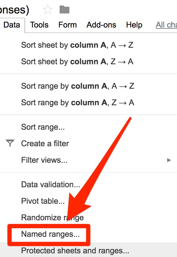
Now I will click on Data from the top menu and select Named ranges….

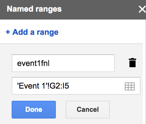
Now I will call these range event1fnl which stands for Event 1 final but you can call it whatever you want just remember to have no spaces.

Now I will do it again for the Event 2, Event 3 and Event 4 worksheets.

Make a new worksheet

Just like in Part 3, we will make one worksheet and then duplicate it for the other teams making the amount of work we have to do a lot less.

To make a new worksheet click on the + icon in the bottom left hand corner.

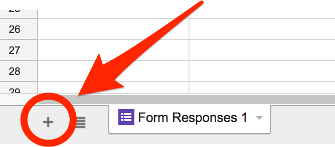
This will create a new sheet and to rename it just double click the tab.

Now we are going to simply type in a bunch of information. No functions yet. So here is how I set up my sheet.

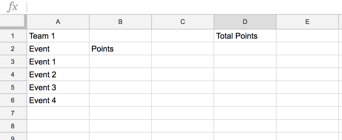
Again, I just typed this information directly into each cell. Now we are ready for some functions. We are only going to use two today: vlookup and sum.

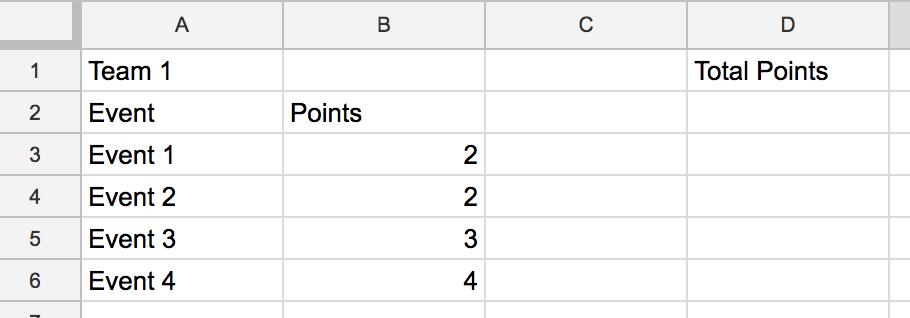
In cell B3 of the Team 1 worksheet we will type this function:

=vlookup(A1,event1fnl,3,0)
Here is what is happening in this function.
vlookup(A1 is looking into cell A1 (which is the team name)
event1fnl is where it will look for the team name
3 means it will look in the third column of the event1fnl data which is how many points were awarded and display that in the cell.
0 means that we want an exact match.

So now in cell B4 we will write this formula:
=vlookup(A1,event2fnl,3,0)

We use event2fnl to show that we want data from Event 2

Then we go on down the list and this is what it should look like.

Believe it or not we are almost done with this post!

sum

No we want to add all those points up. We only have 4 teams and 4 events but imagine you have 7 teams and 14 events! Calculating the totals can take a lot of time. So we will let Google Sheets do the heavy lifting.

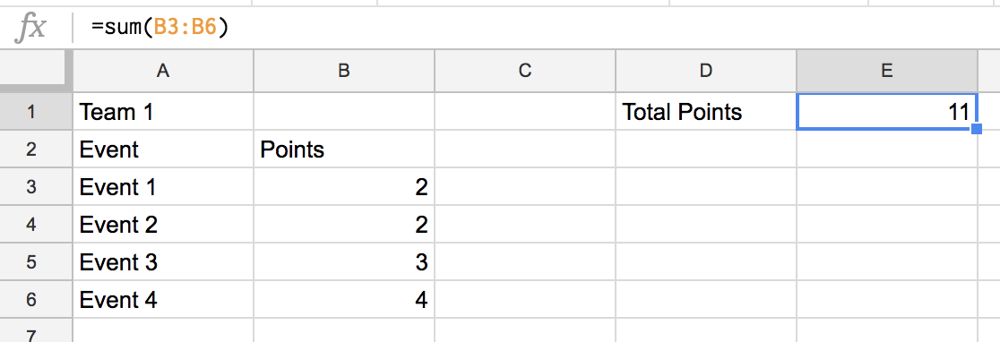
In cell E1 I am going to write this formula – it’s very simple.
=sum(B3+B4+B5+B6)

Now there is another, shorter way to type this formula which is:
=sum(B3:B6)

It does the exact same thing. Some people like the longer way that way they can see exactly what it looks like, but it is totally up to you.

Guess what my friendly reader, we are done with this worksheet!

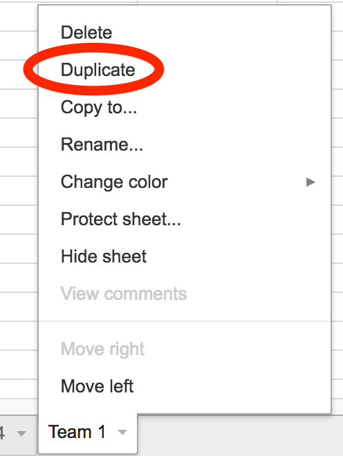
Duplicate

Now we just need to duplicate for each team and then change data in one cell per worksheet. To do this go down to the Team 1 tab at the bottom of the worksheet. Right click the Team 1 tab and then select Duplicate.

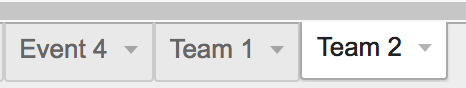
Now rename that worksheet to Team 2.

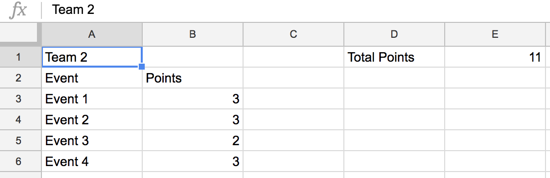
Now you have to make one change, just one and it is easy. In cell A1 on the Team 2 worksheet is the name of the team. Change it from Team 1 to Team 2. That’s it! That’s all that needs to happen and the rest of the worksheet should update.