Google Forms + Form ranger = Event Signup – Part 2

Part 1 was a quick rundown of how we successfully utilized Google Forms to allow parents to sign up for our After School Activities (ASA’s). I didn’t dive into the nitty-gritty when it came to the details about how we utilized the Form Ranger Add-On with Google Forms to make it all work. I made a quickish (it’s about 7 minutes long – I’m out of practice) video to show it, but some people like to see the steps broken down, so keep on reading if that’s you.

Step 1 – Make your Google Form

Pretty simple here. Make sure you are logged into your Google Form and you can head to www.forms.new. This will create a brand new Google Form. You can also do it the old fashioned way of heading over the Google Drive and creating it there. Both work just fine.

For this example we will be asking for a person to select from a number of workshops. Let’s assume that all the workshops are happening on the same day and the same time. If you want to use this over a few days or a week, it can be modified to do that.

On the form I can make a place for people to type their name and then add a multiple choice question. Notice how I do not add any choices – Form Ranger will take care of that for us.

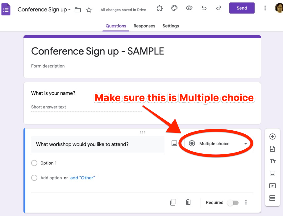
That’s it – we are done with the first step.

Step 2 – Spreadsheet work

Form Ranger requires us to utilize the power of spreadsheets to work. Good news, is that Google Forms stores all its responses in a spreadsheet and here is how you get to that. On the top of the Form you will see options for Questions, Responses, Settings. Click on Responses.

On this page you will want to click on the Google Sheet Icon. This will let you name and it will setup a Google Sheet to store all of the responses.

After it creates the spreadsheet, it will open it up in a new tab. Here is what it should look like.

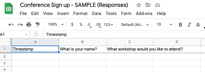
What we need to do is create a new worksheet (spreadsheets can have many, many worksheets). So at the bottom you will see a + sign. Click that and a new worksheet will be created. It is called Sheet2 by default but if you double click the name you can rename it.

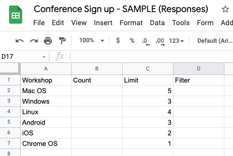
I will rename mine Choices. On the Choices worksheet I will make 4 new column headers. All I do here is literally type those in the cells shown. The headers and their cell reference are listed below.

• Workshops = A1
• Count = B1
• Limit = C1
• Filter = D1

I add in my workshop titles in the Workshops column and I type in the the number of available spaces for each workshop in the Limit column. Again, I am just typing these in, there is no formula to input yet. So here is what the Choices worksheet looks like now.

Step 3 – The functions

Now we are going to do add some functions. If you’ve never done this before it can look and sound intimidating, but it is quite easy. Syntax is important so if you a comma placed somewhere you need to have that comma and so on.

The firs function we are going to add is the Countif function and we will be putting that in the Count column of course. This function will look in a specific area of the data and count what it is looking for. So it will look in the Form Responses worksheet and look for the different workshop names and then count them.

In cell B2 I will type the following:

=countif('Form Responses 1'!C:C,A2)

Here is a breakdown of what all that means:

• = You need this to let the spreadsheet know it is a function
• countif – This will tell the spreadsheet what is happening. In this case it will be counting something
• ‘Form Responses 1’ !C:C – This is where it is looking. It is looking on this worksheet in this column
• , The comma breaks up the parameters of the function. This let’s it know that it is time to move onto what it is looking to count
• A2 – This is what it is looking for. In this specific case it is looking for Mac OS which is what is in cell A2

Here is a quick GIF of me doing this. As you can see it is pretty quick and not too hard. Just don’t forget that comma – that’s really important!

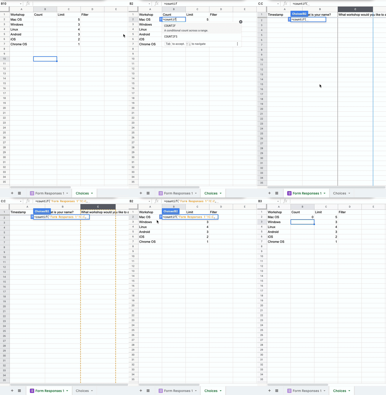
Now, you can type that again for cells B3, B4, and so on or you can do a little trick and replicate it down. In cell B2, click the little square in the bottom right hand part of the cell and drag it down. Google Sheets will take care of the rest.

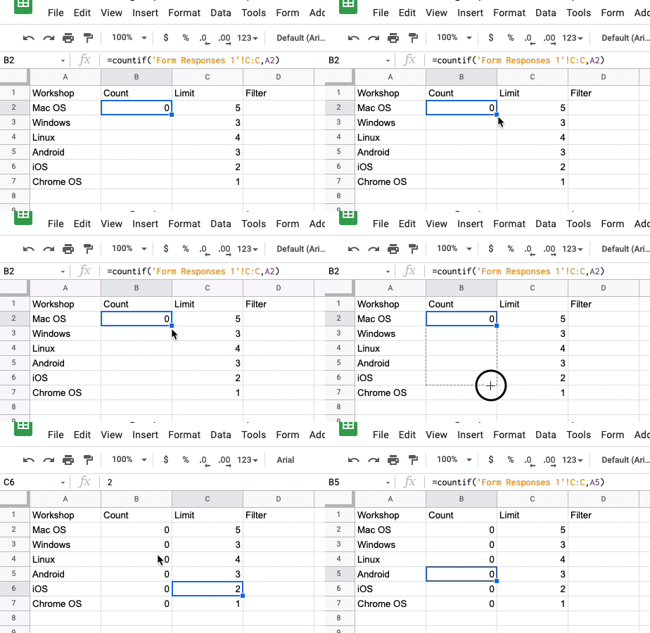
If you see a 0, then you have done it correctly. If you get an error, go back and check your function against mine.

Now onto the other function which is a filter function. We will be writing this function in cell D2.

We are going to tell Google Sheets to compare the numbers in the Count column with the numbers in the Limit column. If those numbers are equal, then it should remove the Workshop from the list. Check out the formula below.

=filter(A2:A7,B2:B7<C2:C7)

Let’s break down this function:

• = You need this to let the spreadsheet know it is a function
• filter – This lets the spreadsheet know we are going to filter out some data to display
• A2:A7 – This is the data on display. The colon in the middle just donates all the cells in between
• , This is crucial as it tells the function that we are moving onto the parameters
• B2:B7<C2:C7 – This is comapring the numbers from the Count column to the numbers in the Limit column and that if the numbers in the Count column are less than the Limit column then they should be displayed.

What should happen is that all the Workshops should show up in Column D. No need to replicate anything – the function will take care of it.

Step 4 – Form Ranger time

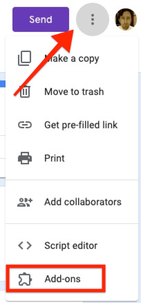
Finally we are ready to add the Form Ranger magic to the form. Head back to the Google Form where you are editing your questions. Then click on the three dots next to your avatar. A drop down menu will appear, select Add-ons

A new window will appear, search for Form Ranger (chances are it will be right there at the top).

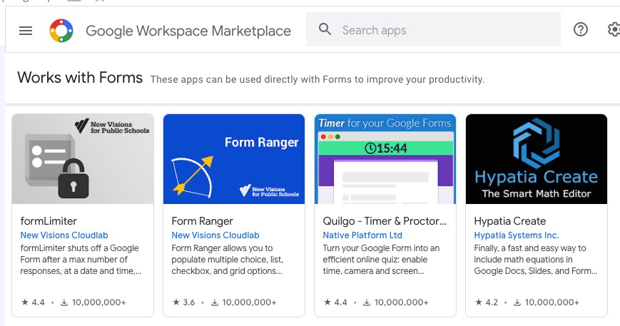
Click on it and go ahead and install it. It will ask you for a number of permissions, go ahead and allow them. Once it is installed, go ahead and close that window.

Now you will see a puzzle piece at the top of your Google Form. Click that and select Form Ranger.

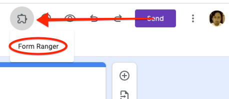
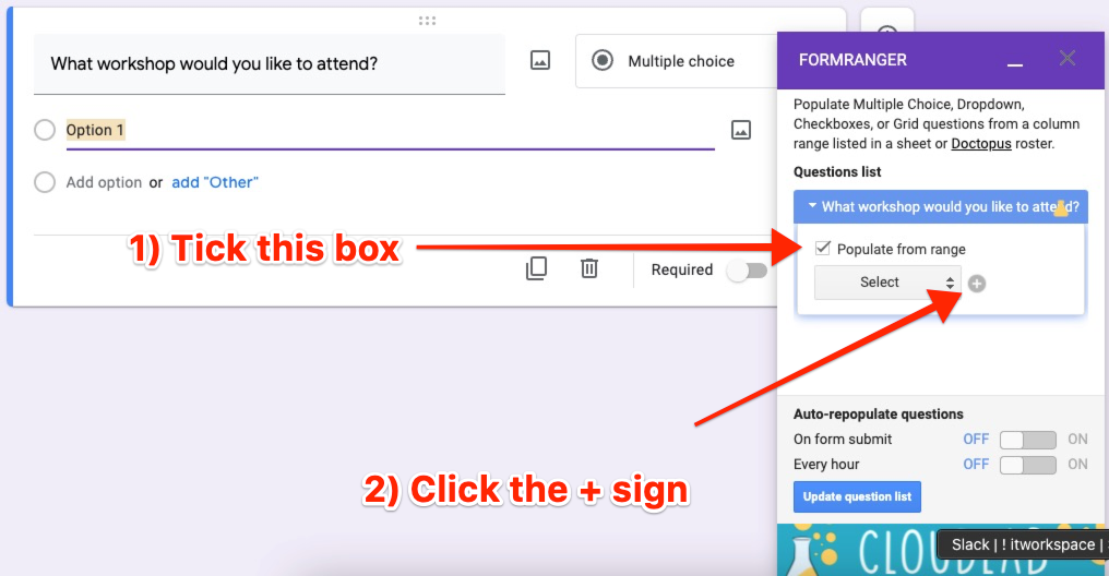
When you do that a small window will appear. Click on Start. The will launch a small window in the bottom left hand corner. What you need to do here is select the question What workshop would you like to attend?

Then tick the box Populate form range and click the + sign next to it.

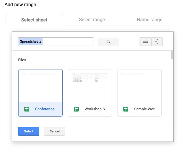
Another new window will pop up, from here select the spreadsheet that is associated with this Google Form (it usually has the same name).

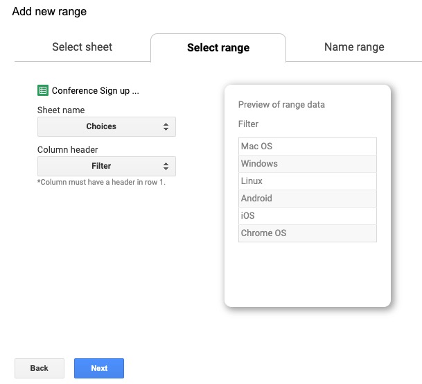
Now it will want some very specific information. You have to tell it which worksheet you want to chose. You will want to the worksheet we named Choices. Then it will want to know the name of the header of what to display. That header is the Filter header.

Click Next and finally it wants you to name the data – name it whatever you want this is something that Form Ranger needs to work behind the scenes. I will call the Range name Filter just to keep it simple. Then click the Save and populate question button and Form Ranger will fill the form with your workshop names! I know this seems like a lot of steps but watch the short GIF below to see how little time this will take you.

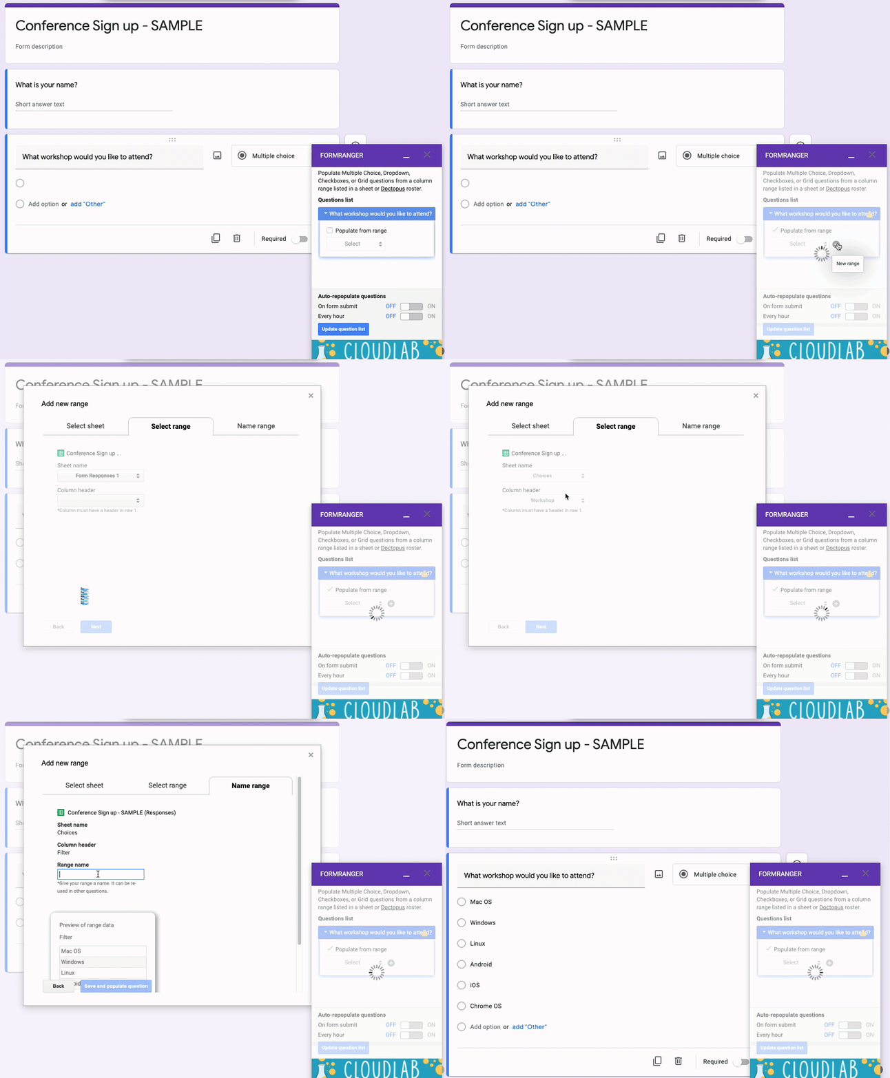
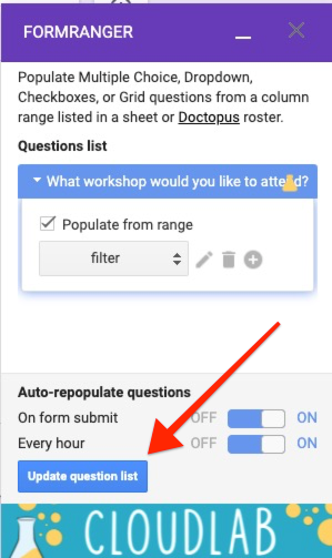
In the Form Ranger window make sure that the On form submit and Every hour option is turned on. This will make sure that the form is updates every time someone submits a form so that the workshop list is properly updating.

We are almost done! All that is left is the testing part and then to distribute it to your community.

Step 5 – Testing

YOU NEED TO DO THIS! In order to make sure the countif and the filter functions are working you need to test. The worst thing you can do is set this up, have a limit of 15 spaces and then find out 35 people have signed up for a workshop.

I like to test in a different browser. I work in Chrome and usually test in Firefox, Edge or Safari – basically any browser that a Google account is not logged into. So to get the link for the Google Form and open it in our different browser. To get the link look for the weird eye ball at the top of your Google Form. This is the link to the actual live form.

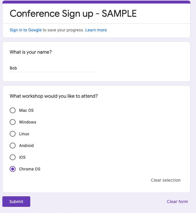
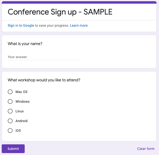
Chrome OS is gone! Yes! Now we test again and again picking each workshop at least once.

Now head back over to your spreadsheet with the responses. Go to the Choices worksheet and make sure that it is counting correctly.

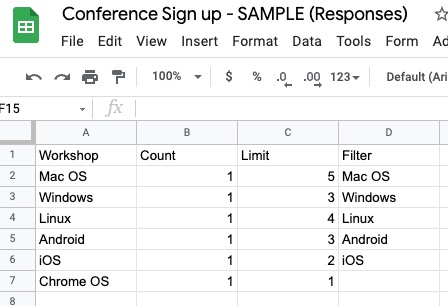
Yep – that is looking good. It is counting correctly and the Chrome OS has been removed in the Filter column. We are nearly ready to go live with this awesome form!

Step 6 – Going live

We need to remove our test responses. This is a three step process. Step one is to go to the Form in the Responses section you will need to Delete all responses. Check out the GIF below to see how this is done.

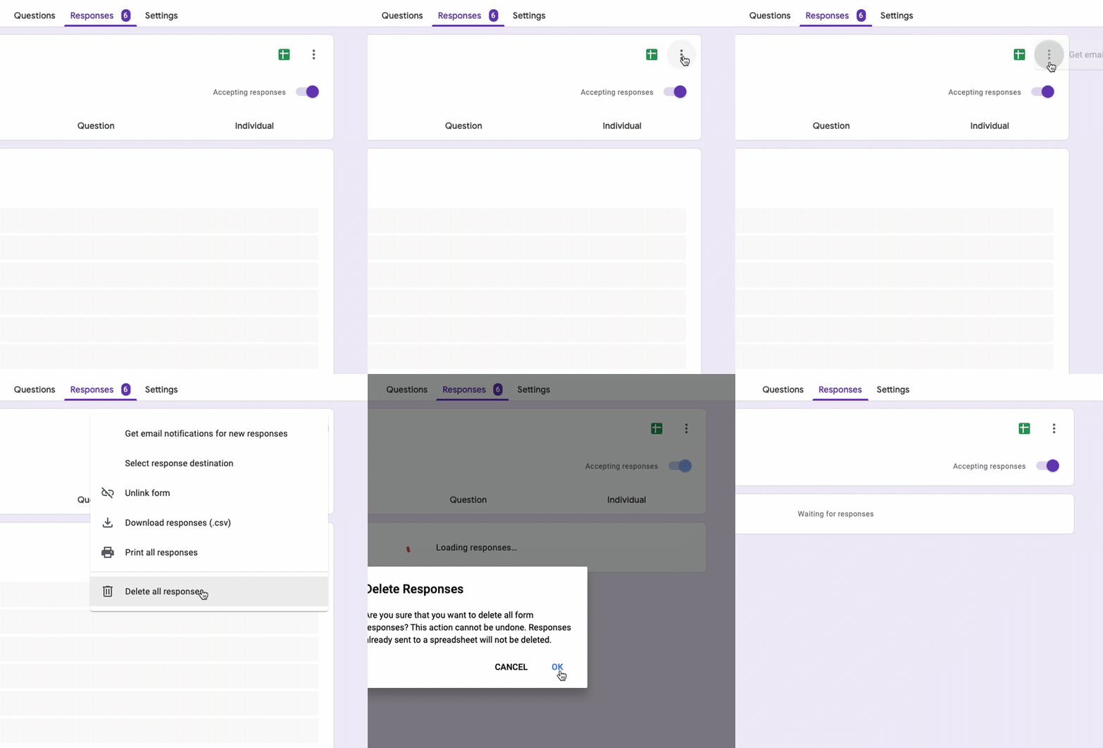
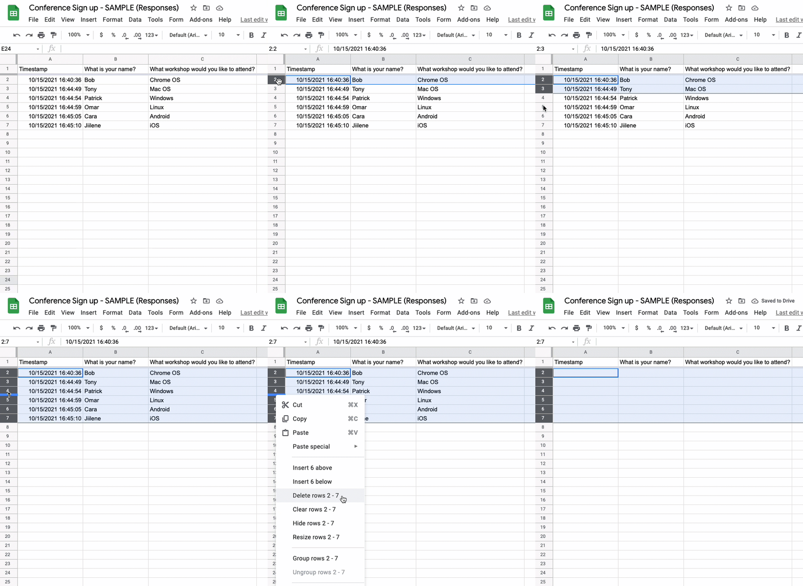
Now we need to go over to the spreadsheet itself and delete all the rows that have information in it. Again, check out the GIF below to see how that is done.

Finally you will need to go to Form Ranger and click the Update question list button. This forces the form to look back at the Filter column. It will see that Chrome OS is now back in the list and re-add it to the multiple choice question.

That will do it. Now you are ready to send the link out in an email to your community.

What if…

A question I usually get is what if there is one spot left and two people start the form at the same time. Both will see the workshop is available – what happens? I’ve run into this and I can show what happens. The slower of the two to submit will get this error on their form itself.

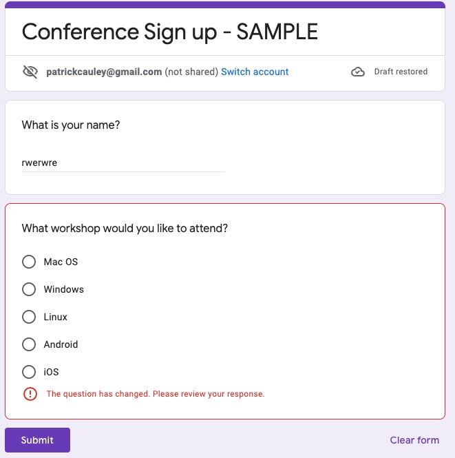
It will not allow them to submit it. I’ve never seen Form Ranger allow too many responses . . .ever. I ‘m not saying it’s impossible but I find it very unlikely.

Going further

This is just the start. You can actually go a little further with this idea. I recommend to Collect email addresses and always send responders a copy of their responses. You can turn this feature on in the Settings section of your form.

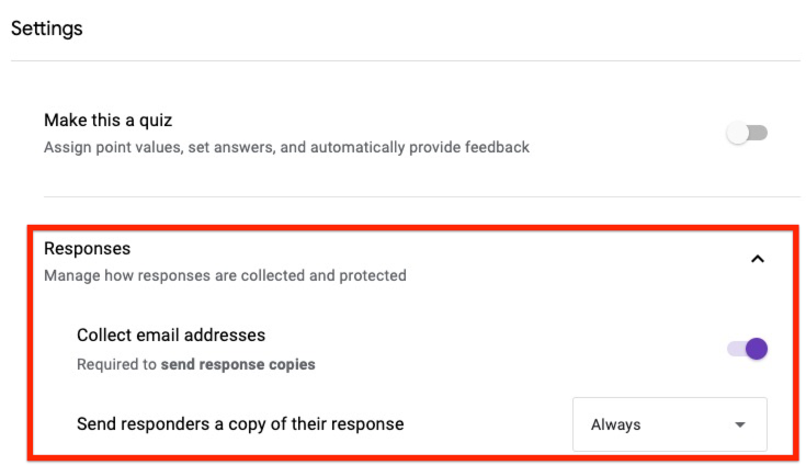
That way people will get an email “confirmation” of what they have selected. It makes them feel fuzzy and confident that everything is OK.

You can also make rosters for each workshop. To do this I make a worksheet for each workshop and utilize the Query function. I wrote about it here and made a video below.

This is just the tip of the iceberg- there are plenty of other directions to go using the Google Form + Form Ranger setup. Just play around and find out what works for you!

Source: IT Babble Blog and Podcast